
The group consists of the following sections:
- Well Information
- Wellbore
- Fluid
- Inflow
Parameters in these sections do not depend on the well lift type and are essential for accurate calculations.
Well Information
The Well information section provides general information about the well. It consists of two tabs:
- Well data
- Multiphase flow parameters
Well Data
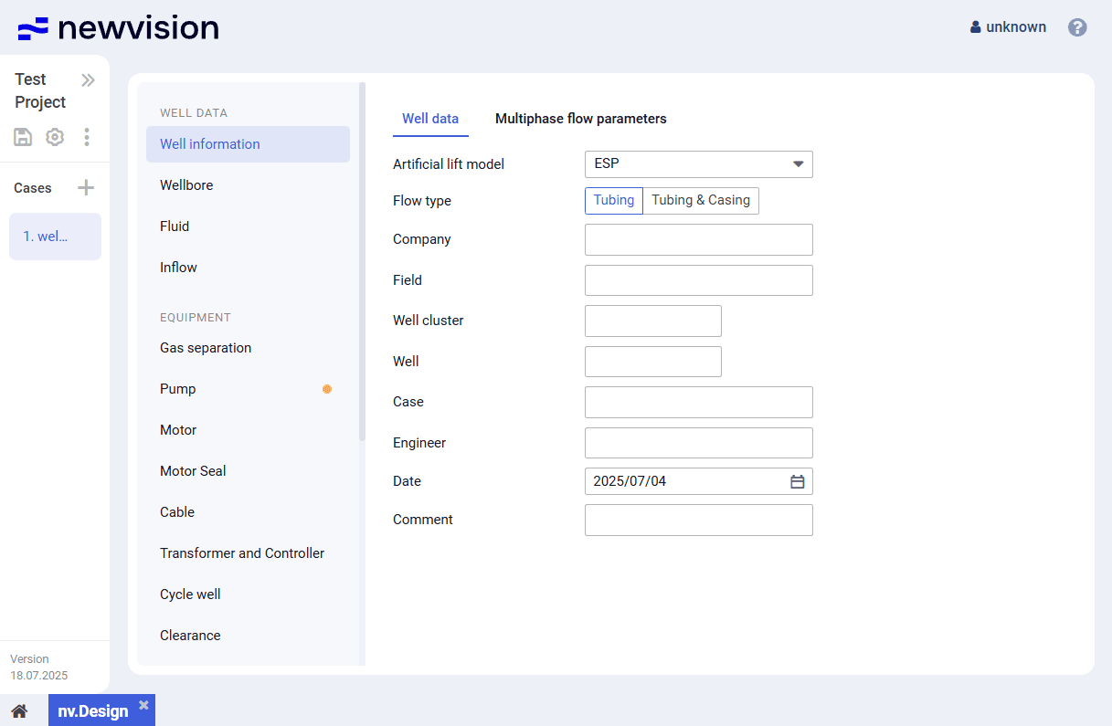
On the Well data tab, you can select the well lift type and enter general information about the well, such as company name, field name, well number, etc.
Multiphase Flow Parameters
On the Multiphase flow parameters tab, you can select correlations used for the tubing multiphase flow and configure their application conditions.
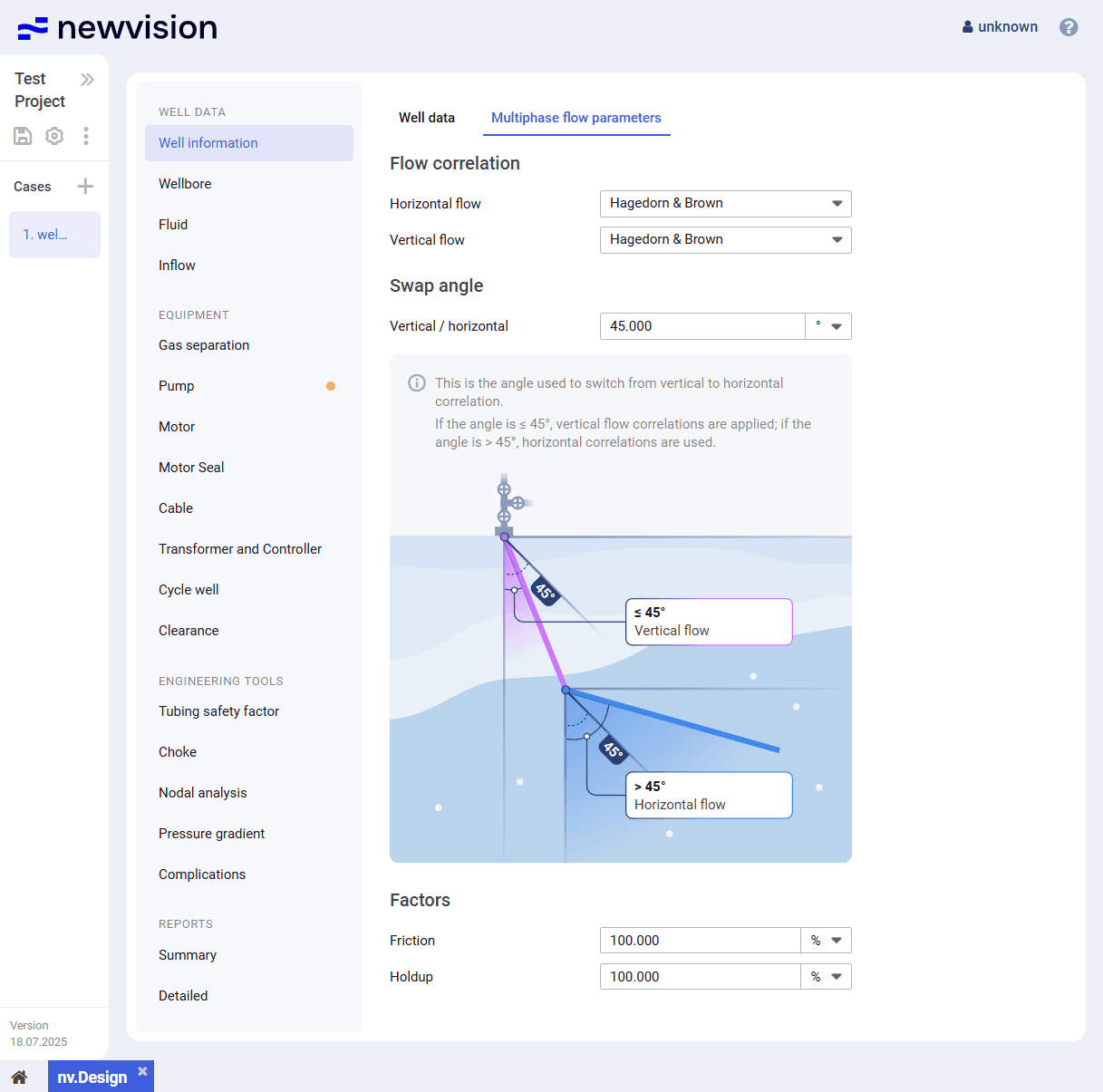
The tab contains the following parameter groups:
- Flow correlation
- Angle of transition between flows
- Factors
Flow Correlation
In this group, you can select correlations that will be used for the horizontal and vertical flow calculations. For details on the available correlations, see .
Angle of Transition Between Flows
In this group, you can set the threshold inclination angle at which the system switches between horizontal and vertical flow correlations.
Below the field with the angle value, a simplified flow scheme is displayed. It visualizes horizontal and vertical flows and the selected transition angle.
 | Note |
Factors
In this group, you can specify the friction and hold-up factors. They can be used to adjust pressure loss calculations in the wellbore:
- Friction factor affects frictional losses (ΔPf).
- Hold-up factor affects the hydrostatic gradient (ΔPa).
The total pressure loss is calculated using the following formula:
ΔP = (friction factor ΔPf) + (hold-up factor⋅ΔPa) + ΔPg
ΔP = (friction factor⋅ΔPf) + (hold-up factor ΔPa) + ΔPg
| Note |
The default value for both friction and hold-up factors is 100%. You can modify it in calibration and testing purposes.
Multiphase Flow Correlations
On the Multiphase flow parameters tab of the Well information section, the following multiphase flow correlations can be selected:
Moody
The Moody correlation is used to calculate friction factors and pressure losses in single-phase flows of gas or liquid, based on Reynolds number and relative pipe roughness. While it was originally developed for single-phase conditions, it is often incorporated into multiphase models to estimate friction factors in each phase separately.
Typical data ranges:
- Temperature: 4°C – 177°C
- Pressure: 0.1 bar – 689 bar
Gray
The Gray correlation accounts for the influence of gas-liquid interaction in multiphase flow, specifically designed for pressure drop estimation in gas-lift operations and vertical wellbores. It is well suited for calculating bottomhole pressure and tubing performance where the gas-liquid ratio significantly affects flow behavior.
Typical data ranges:
- Temperature: 4°C – 150°C
- Pressure: 6.89 bar – 345 bar
- Gas-liquid ratio: Broad range typical for gas-lift systems
Poettmann-Carpenter
The Poettmann-Carpenter method was one of the first empirical models to incorporate the effects of two-phase flows in vertical wells. It estimates pressure losses in tubing based on flow rates and pipe dimensions, enabling basic evaluation of artificial lift performance and production behavior.
Typical data ranges:
- Temperature: 4°C – 177°C
- Pressure: 0.1 bar – 689 bar
Orkiszewski
The Orkiszewski correlation is widely applied in vertical multiphase flow modeling. It accounts for flow regime transitions (bubbly, slug, annular, segregated) and includes corrections for different flow patterns. This makes it valuable for pressure drop predictions in well design and production optimization.
Typical data ranges:
- Temperature: 4°C – 177°C
- Pressure: 0.1 bar – 689 bar
Griffith
The Griffith correlation is applied to vertical two-phase flows, particularly in wellbores. It considers gas-liquid interaction and offers a simplified method to calculate pressure losses based on mixture properties and flow regime assumptions.
Typical data ranges:
- Temperature: 4°C – 177°C
- Pressure: 0.1 bar – 689 bar
Duns & Ros
The Duns & Ros correlation evaluates pressure losses in vertical and inclined multiphase flow, accommodating various flow regimes including bubbly, slug, and annular. It provides accurate results for high gas-liquid ratio conditions that are often encountered in oil wells.
Typical data ranges:
- Temperature: 4°C – 177°C
- Pressure: 0.1 bar – 689 bar
Beggs & Brill
The Beggs & Brill correlation was developed for multiphase flows in pipelines with different inclination angles. It offers regime-specific calculations for pressure losses in horizontal, vertical, and inclined sections. This correlation is widely adopted due to its flexibility and applicability to field-scale models.
Typical data ranges:
- Temperature: 4°C – 177°C
- Pressure: 0.1 bar – 689 bar
Aziz
The Aziz model is designed for predicting multiphase pressure gradients in inclined and horizontal pipes. It captures complex gas-liquid interactions and adjusts for pipe angle, making it effective in pipelines and horizontal wellbores.
Typical data ranges:
- Temperature: 4°C – 177°C
- Pressure: 0.1 bar – 689 bar
Ansari
The Ansari correlation offers a mechanistic approach for predicting pressure drop, velocity, and flow distribution in vertical and inclined wells. It integrates flow regime transitions and detailed physical modeling to make it suitable for high-accuracy production system simulations.
Typical data ranges:
- Temperature: 4°C – 177°C
- Pressure: 0.1 bar – 689 bar
Hagedorn-Brown
The Hagedorn-Brown correlation is one of the earliest and most widely used models for vertical two-phase flows in oil wells. It enables reliable calculation of pressure losses based on well depth, fluid rates, and tubing diameter, serving as a benchmark for many commercial software implementations.
Typical data ranges:
- Temperature: 4°C – 177°C
- Pressure: 0.1 bar – 689 bar
Wellbore
The Wellbore section provides information about the downhole equipment, well profile, and heat transfer. It consists of three tabs:
- Wellbore configuration
- Deviation survey
- Heat transfer
Wellbore configuration
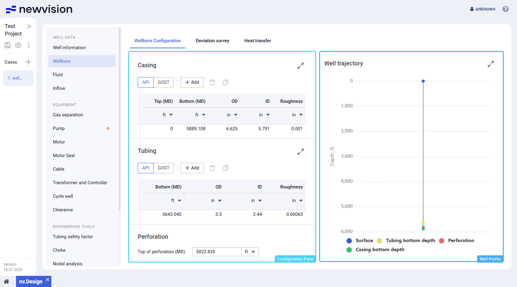
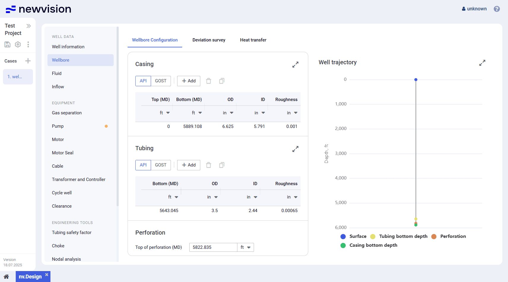
On the Wellbore Configuration tab, you can configure tubing and casing parameters, such as their top and bottom depths (MD), number of stages, and diameters.
The tab consists of two panes:
- Configuration pane in the left part of the tab.
- Well profile in the right part of the tab.
Configuration Pane
The pane contains three groups of parameters: Casing, Tubing, and Perforation.
The Casing and Tubing groups contain tables with corresponding parameters. Each row in the table corresponds to one casing or tubing stage.
Both tables provide the following controls:
API/GOST
Provides the ability to select the set of standard pipe sizes, API (American Petroleum Institute standard) or GOST (Russian national standard), that prescribes the tubing and casing outer and inner diameters.
Add ( )

Adds a new row to the table for entering the casing or tubing stage parameters at the specified depth. For details, see Configuring Casing and Tubing Data.
You can enter data to the tables manually or paste it to a new row from another source using the Ctrl+V shortcut. The source table must have the same column configuration as the target one. The pasted entries are automatically sorted by depth.
For example, you can try copying the data from the following table:
Top (MD) | Bottom (MD) | OD | ID |
0 | 8690 | 7 | 6.276 |
8400 | 11320 | 4.5 | 3.92 |
0 | 7150 | 2.875 | 2.441 |
| Note |
Delete ( )

Deletes the selected row from the table.
Clone ( )

Creates a copy of the selected row.
Expand ( ) / Collapse ( )


Expands the parameter group to full screen or collapses it back to the original size.
The Perforation group contains only one parameter, Top of perforation (MD).
Well Profile
The pane contains the well profile that is built based on the data entered in the left part of the section (see description above).
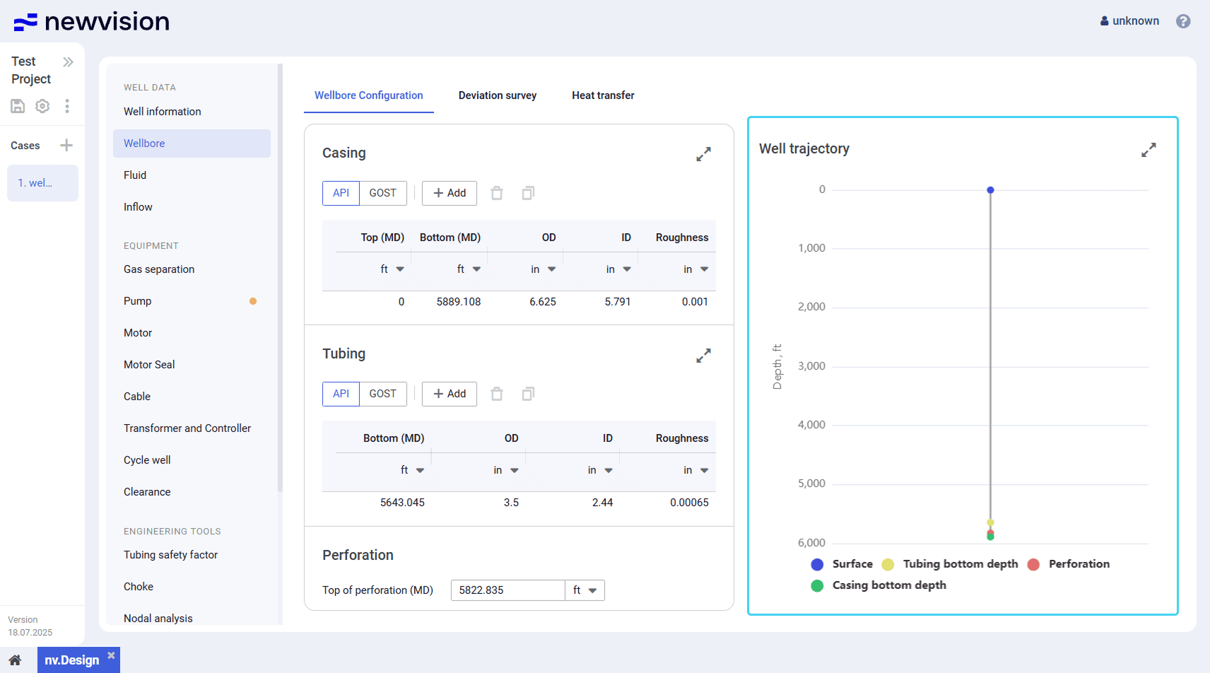
On the profile, depths are displayed as markers of different color.
To show or hide a marker, click its name under the profile.
You can also expand the pane to full screen or collapse it back to the original size using the Expand ( ) / Collapse ( ) buttons located in the upper-right corner of the pane.
Configuring Casing and Tubing Data
To configure the well tubing and casing parameters, perform the following actions:
- Open the nv.design module.
For details on navigation in the system, see System Interface. - In the left part of the working area, in the list of the module sections, click Wellbore.
To the right of the list, the Well Configuration tab opens.
- In the Casing parameter group, select the standard for outer and inner diameters of the casing: API or GOST.
- Add new entries to the table. You can do it in the following ways:
- To add a new entry, perform the following actions:
Above the table, click Add ( ).
A new row appears in the table.- In the new row, double-click values in the Top (MD) and Bottom (MD) columns and enter the desired values.
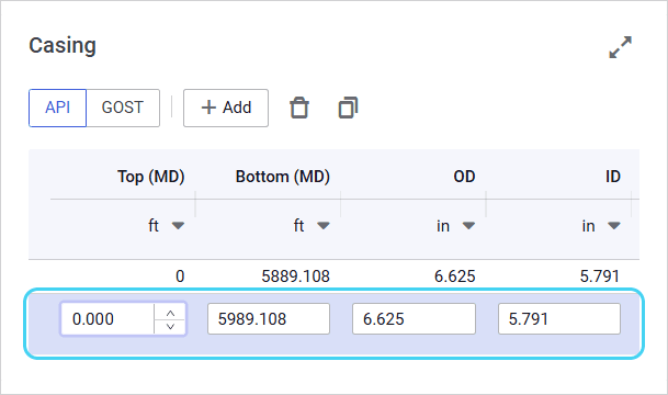
- Double-click values in the OD and ID columns and select the desired outer and inner diameters from the lists.
To create a copy of an existing entry, select the entry that you want to copy in the table, and then, above the table, click Duplicate ( ).
The copied entry appears in the table.- To paste a row with data from another table, copy it to the clipboard, select any entry in the table, and then press Ctrl+V.
The copied entry appears in the table.
| Note |
- Entries in the table are automatically sorted by the Bottom (MD) value.
- Repeat Steps 3–4 for the Tubing parameter group.
In the right part of the Well Configuration tab, the well profile is displayed. - (Optional)
- To edit an entry, double-click the desired value and make necessary changes.
To delete an entry, select it in the table, and then, above the table, click Delete ( ).
To save changes, in the left part of the module, click Save ( ) under the name of the current project.

Deviation survey
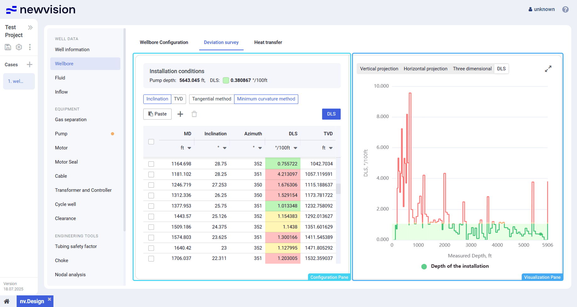
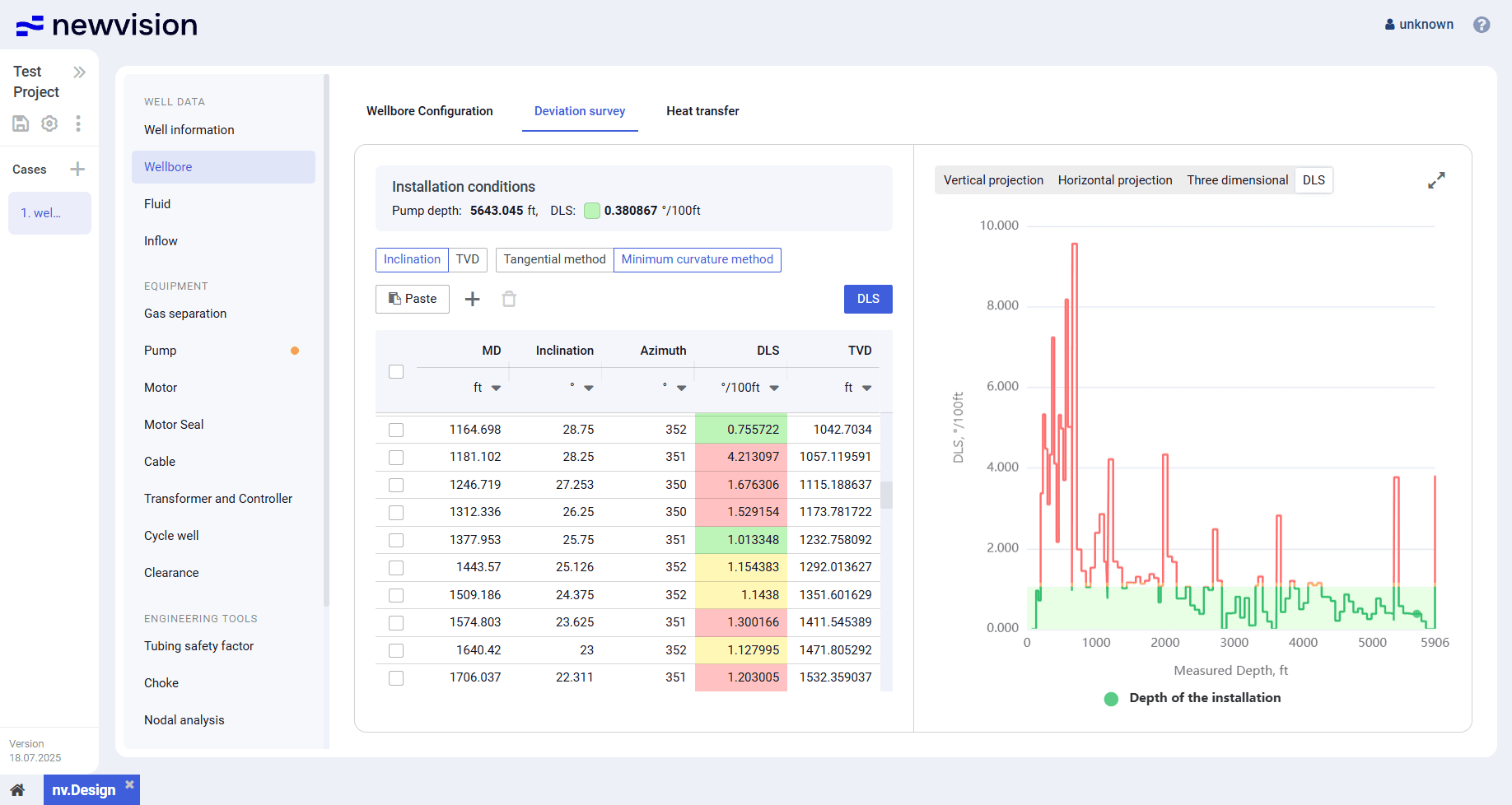
On the Deviation survey tab, you can build vertical, horizontal, dogleg severity (DLS), and 3D projections of the well.
The tab consists of two panes:
- Configuration pane in the left part of the tab.
- Visualization pane in the right part of the tab.
Configuration Pane
The pane contains a table with the well directional survey data required for calculation. For details on how to enter the data and run a calculation, see Running Deviation Survey Calculation.
At the top of the pane, the installation conditions are displayed:
- Pump depth value equals the tubing bottom measured depth taken from the Wellbore configuration tab.
- DLS value corresponds to the dog leg severity at the pump setting depth. If there is no data for this very depth, the next available value is taken.
The color of the square to the left of the DLS value indicates if it is feasible to install the pump at this depth: a green square means that the maximum DLS value is withing the allowable range, a red one means that the maximum allowable value is exceeded. This value can be configured in the ESP depth setting determination window. For details, see Configuring DLS.
Below the Installation conditions area, the following controls are available:
Inclination / TVD
Provides the ability to select the parameter based on which the calculation will be performed.
In the table, values of the selected parameter are entered manually. Values of the other parameter are calculated automatically.
Tangential method / Minimum curvature method
Provides the ability to select the calculation method:
- The Tangential method assumes constant inclination and azimuth between survey points. Is simpler but less accurate.
- The Minimum curvature method models the well as a smooth arc and provides higher accuracy, especially over longer intervals.
By default, the Minimum curvature method is used as it offers the most reliable results for most wellbore profiles.
Paste ( )

Pastes data from the clipboard to a new row in the table.
Alternatively, to paste data, you can use the Ctrl+V shortcut.
| Note |
Add ( )
Adds a new row to the table for entering the deviation survey data. For details, see Running Deviation Survey Calculation.
Delete ( )

Deletes the selected rows from the table.
To select a row, select the corresponding check box in the leftmost column of the table.
DLS
Opens the ESP depth setting determination window where you can calculate the maximum allowable DLS values based on the ESP length and outer diameter. For details, see Configuring DLS.
In the table, values in the first three columns are editable. Values in the other two are calculated automatically.
In the DLS column, the following color indication is used based on the maximum allowable DLS:
- Green fill: The value is well below the critical value and no actions are required.
- Yellow fill: The value is 0,89-0,9 of the critical value and requires attention.
- Red fill: The value is greater than the critical value and must be fixed.
Visualization Pane
The pane provides the following types of the well projections distributed on the corresponding tabs:
- Vertical projection
- Horizontal projection
- DLS
- 3D projection
 | Important |
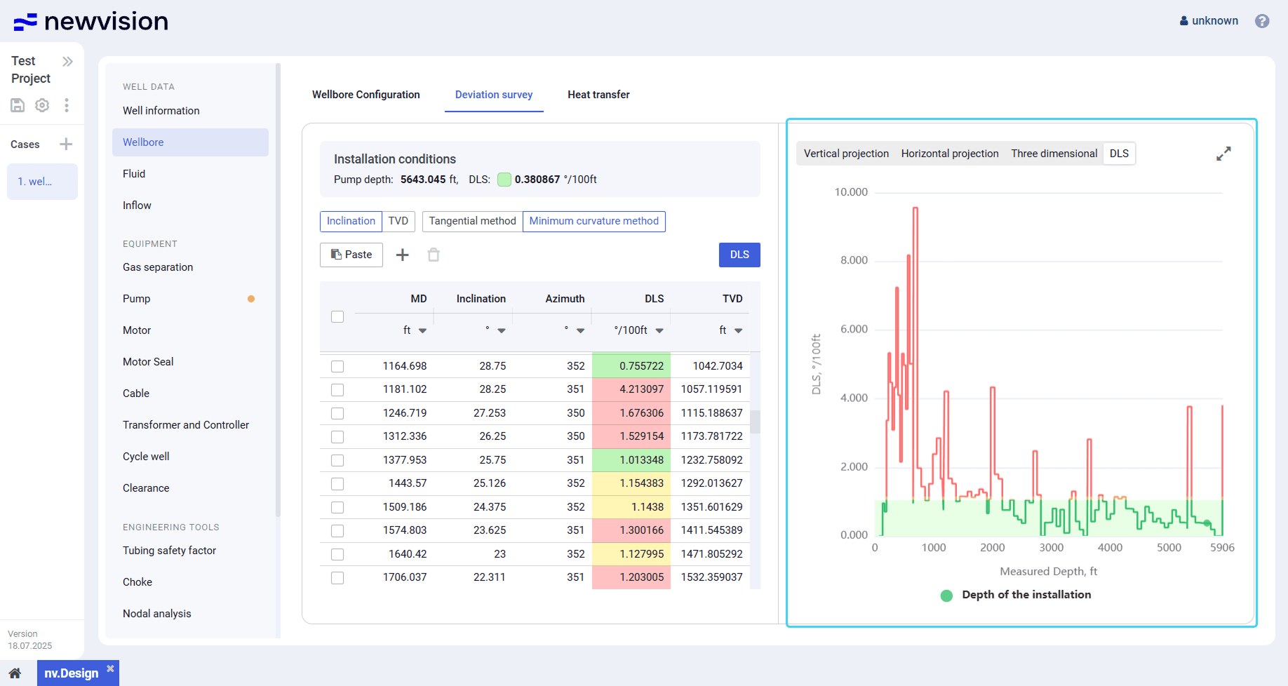
On the DLS tab, sections suitable for equipment installation are highlighted with a green fill.
On other projections, depths are displayed as markers of different color.
To show or hide a marker, click its name under the profile.
You can also expand the pane to full screen or collapse it back to the original size using the Expand ( ) / Collapse ( ) buttons located in the upper-right corner of the pane.
Configuring DLS
To configure the well tubing and casing parameters, perform the following actions:
- Open the nv.design module.
For details on navigation in the system, see System Interface. - In the left part of the working area, in the list of the module sections, click Wellbore, and then go to the Deviation survey tab.
- At the top of the pane in the left part of the section, click DLS.
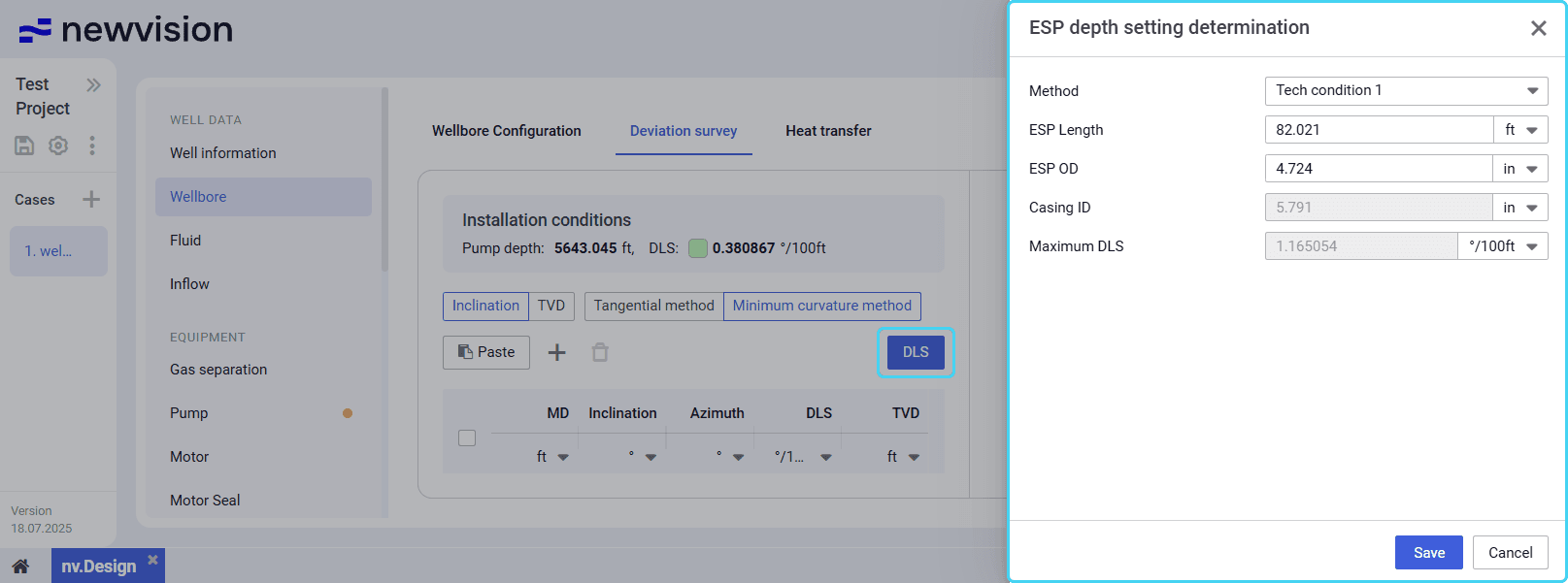
The ESP depth setting determination window opens in the right part of the section.
- In the window that appears, perform the following actions:
- From the Method list select the calculation method: Tech Condition 1 (less strict) or Tech Condition 2 (stricter).
- (Optional) Edit values in the ESP Length and ESP OD fields.
Values in the Casing ID and Maximum DLS fields are calculated automatically. - At the bottom of the window, click Save.
To save changes, in the left part of the module, click Save ( ) under the name of the current project.
Running Deviation Survey Calculation
To configure deviation survey parameters and run a calculation, perform the following actions:
- Open the nv.design module.
For details on navigation in the system, see System Interface. - In the left part of the working area, in the list of the module sections, click Wellbore, and then go to the Deviation survey tab.
- At the top of the pane in the left part of the section, select the parameter based on which the calculation will be performed: Inclination or TVD.
| Note |
- To the right of the parameters selected at the previous step, select the calculation method:
- The Tangential method assumes constant inclination and azimuth between survey points. Is simpler but less accurate.
- The Minimum curvature method models the well as a smooth arc and provides higher accuracy, especially over longer intervals.
| Note |
- Above the table, click DLS and configure the maximum allowable dog leg severity. For details, see .
- Add new entries to the table. You can do it in the following ways:
- To add a new entry, perform the following actions:
Above the table, click Add ( ).
A new row appears in the table.- In the new row, double-click values in the first three columns and enter the desired values.
Values in the other two columns are calculated automatically.
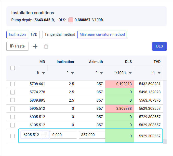
To paste a row with data from another table, copy it to the clipboard, and then, above the table, click Paste ( ), or press Ctrl+V.
The copied entry appears in the table.
| Note |
(Optional) To delete an entry from the table, select it, and then, above the table, click Delete ( ).
- Ensure that in the Installation conditions area above the table, the color of the square to the left of the DLS value is green. If it is red, make changes to the parameter values.
- When the configuration is completed and there are no errors, in the right part of the tab, the well projections are displayed.
- On the DLS tab, sections suitable for equipment installation are highlighted with a green fill.
To save changes, in the left part of the module, click Save ( ) under the name of the current project.
Heat transfer
On the Heat Transfer tab, you can model the temperature distribution along the wellbore.
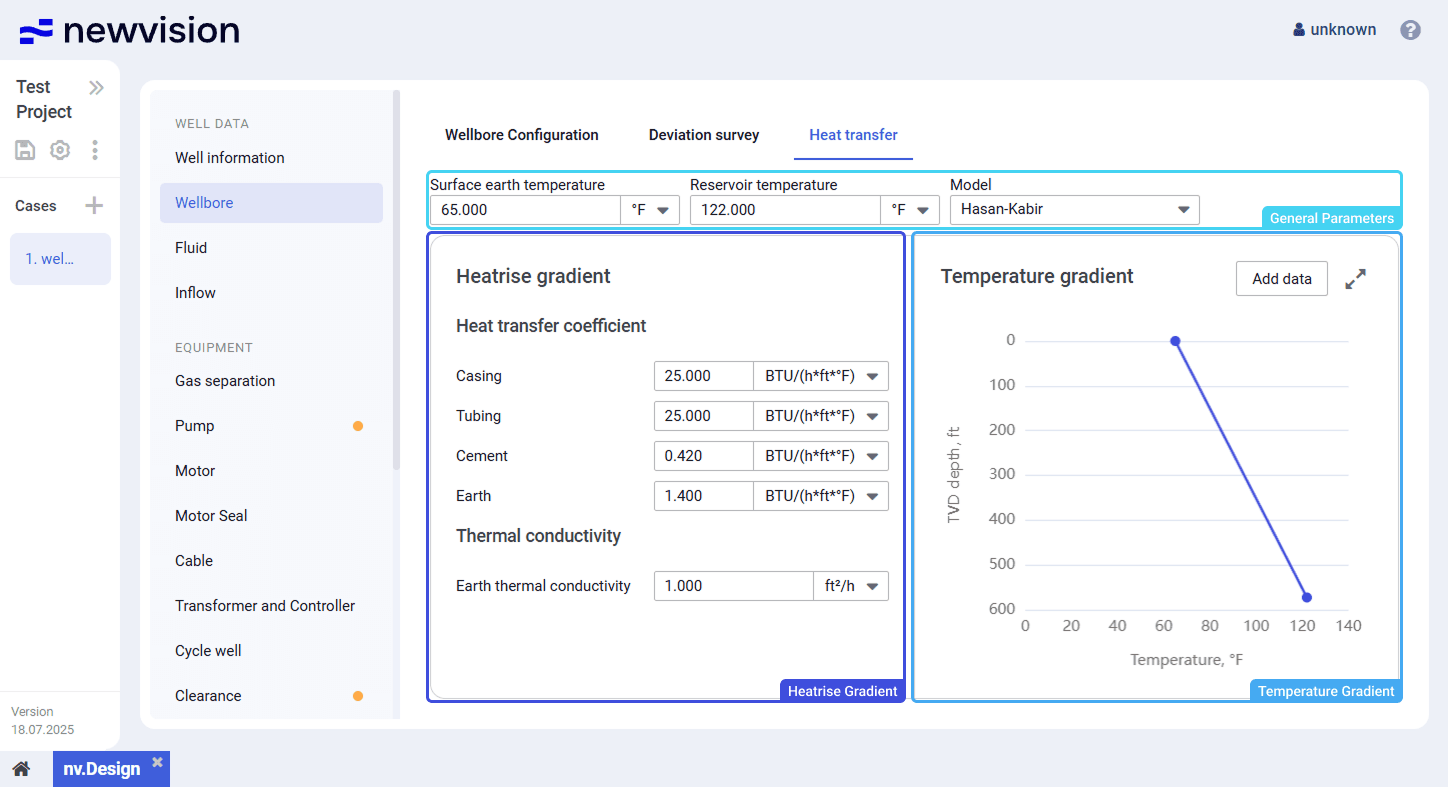
The tab consists of the following parts:
- General parameters at the top of the tab.
- Heatrise gradient pane in the left part of the tab.
- Temperature gradient pane in the right part of the tab.
General Parameters
General parameters are required for the temperature gradient modeling.
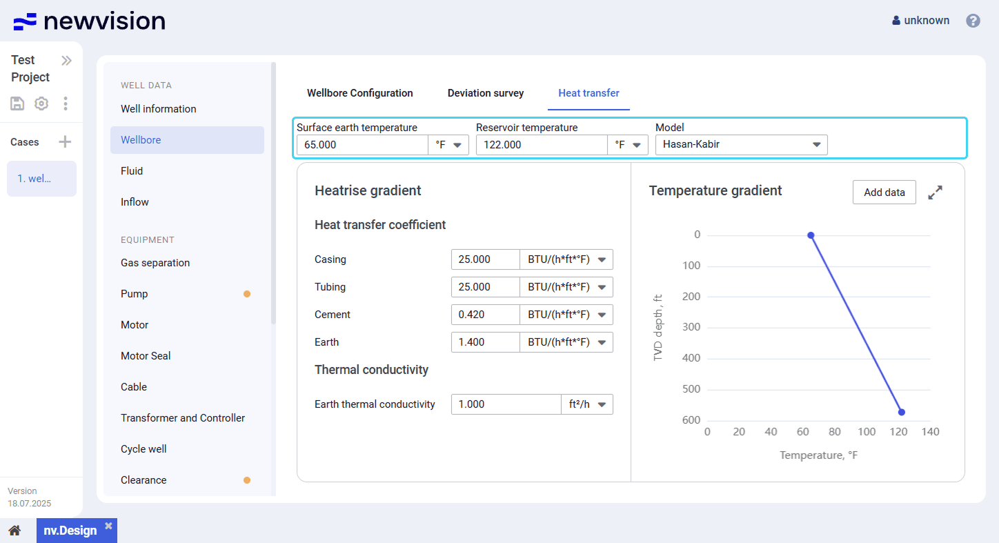
There, you need to specify the Surface earth temperature and Reservoir temperature values and select the calculation model from the Model list.
Two calculation models are available:
- Hassan-Kabir: Provides more accurate estimates as it takes into account heat transfer coefficients of the well casing, tubing, cement, and formation, as well as thermal conductivity of the surrounding formation.
This method is based on a semi-analytical model developed by Hasan and Kabir, which solves the energy balance equations to estimate fluid and formation temperatures during steady-state or transient flow in the wellbore. - Rough Approximation: Provides less accurate but faster estimates. It requires fewer input parameters and uses only a general (lumped) heat transfer coefficient. This model is suitable for quick estimations or cases where detailed thermal data is unavailable. It generates a simplified temperature profile along the wellbore.
| Important |
Heatrise Gradient
The pane contains well parameters that affect temperature distribution along the wellbore.
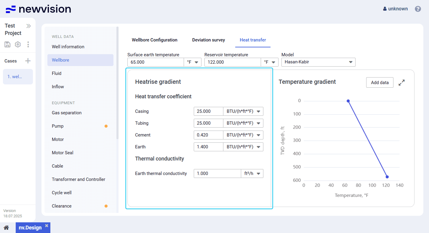
Depending on the selected model (see description above), different sets of parameters are available.
If the Hassan-Kabir model is selected, the pane contains two parameter groups:
- Heat transfer coefficient
- Thermal conductivity
If the Rough Approximation model is selected, only the Overall heat transfer coefficient value can be specified.
Temperature Gradient
The pane contains a chart representing the well temperature profile constructed based on the input data and selected calculation model.
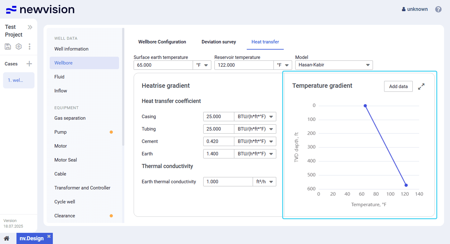
To improve the profile accuracy, you can add more information about the wellbore temperature at different depths. For details, see Adding Well Test Data.
You can also expand the pane to full screen or collapse it back to the original size using the Expand ( ) / Collapse ( ) buttons located in the upper-right corner of the pane.
Configuring Heat Transfer Parameters
To configure the well heat transfer parameters, perform the following actions:
- Open the nv.design module.
For details on navigation in the system, see System Interface. - In the left part of the working area, in the list of the module sections, click Wellbore, and then go to the Heat transfer tab.
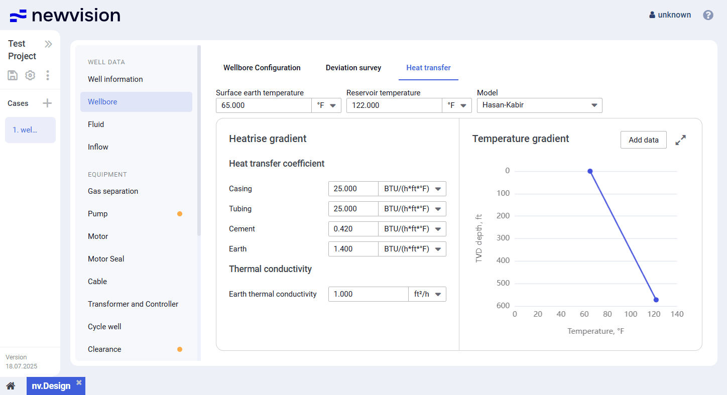
- At the top of the tab, in the Surface earth temperature and Reservoir temperature fields, enter the desired values.
- From the Model list, select the calculation model. For details, see .
- (Optional) In the Heatrise gradient pane, edit values of the desired parameters.
| Note |
- (Optional) To enhance the accuracy of the well temperature profile, in the upper-right corner of the section, click Add data and enter available temperature data at different well depths. For details, see Adding Well Test Data.
- After the configuration is completed, in the Temperature gradient pane, view the resulting temperature profile.
To save changes, in the left part of the module, click Save ( ) under the name of the current project.
Adding Well Test Data
To add temperature data obtained during the well tests, perform the following actions:
- Open the nv.design module.
For details on navigation in the system, see System Interface. - In the left part of the working area, in the list of the module sections, click Wellbore, and then go to the Heat transfer tab.
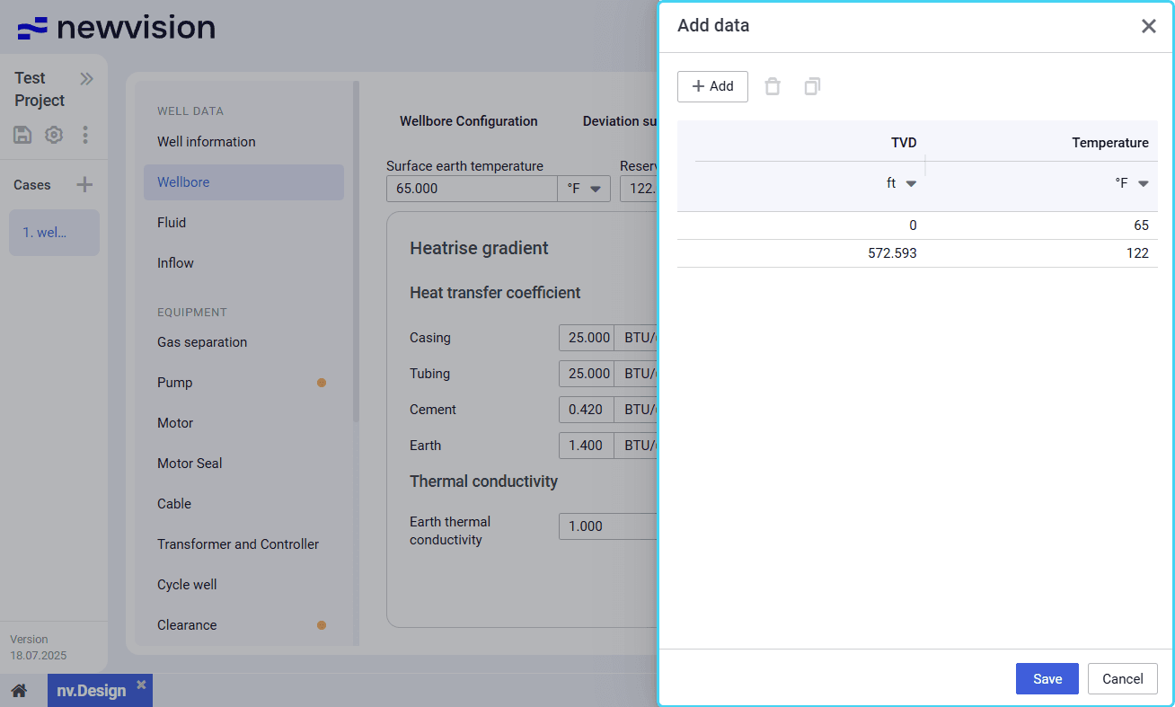
- At the top of the pane, in the right part of the section, click Add data.
The Add data window opens in the right part of the section.
| Note |
Add new entries to the table. You can do it in the following ways:
To add a new entry, above the table, click Add ( ), and then, in the new row, double-click values in the TVD and Temperature columns and enter the desired values.
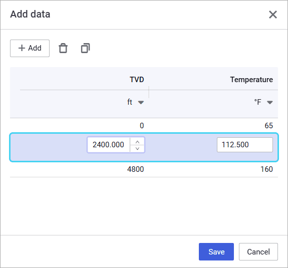
To create a copy of an existing entry, select the entry that you want to copy in the table, and then, above the table, click Duplicate ( ).
The copied entry appears in the table.
- (Optional)
- To edit an entry, double-click the desired value and make necessary changes.
To delete an entry, select it in the table, and then, above the table, click Delete ( ).
To save changes, in the left part of the module, click Save ( ) under the name of the current project.
Fluid
The section provides information about the PVT properties of oil, water, and/or gas. It consists of two tabs:
- Fluid
- Correlations
Fluid
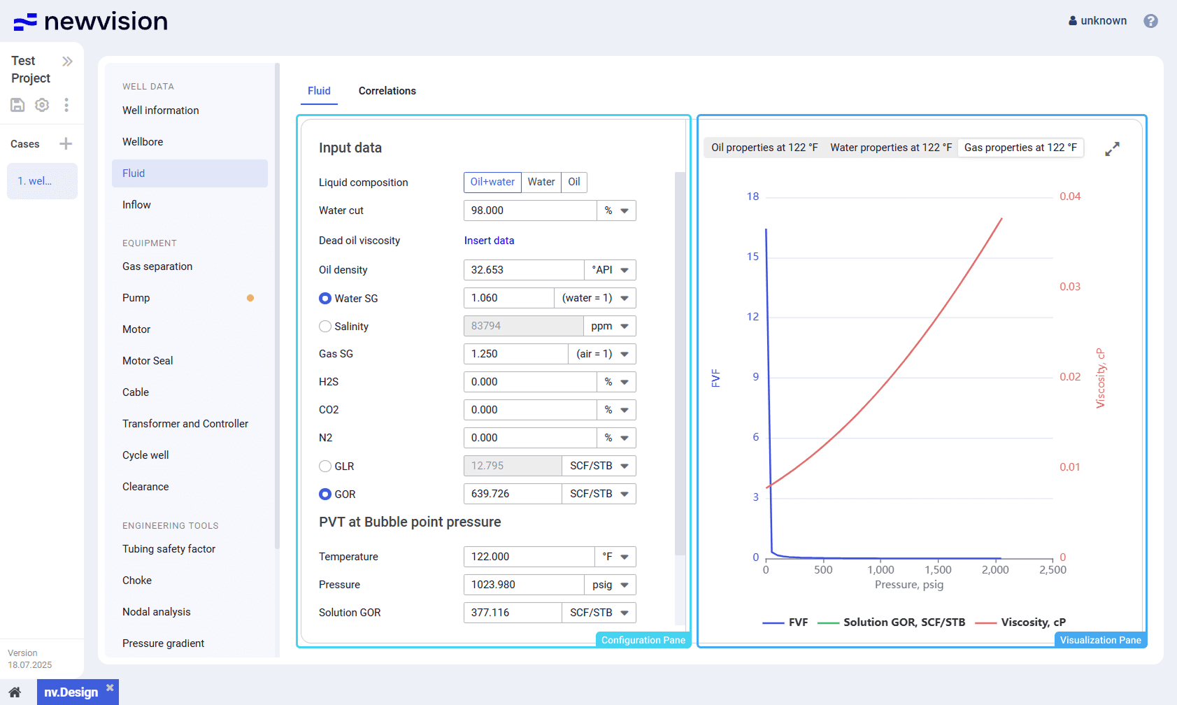
On the Fluid tab, you can configure PVT properties of the well fluid.
The tab consists of two panes:
- Configuration pane in the left part of the tab.
- Visualization pane in the right part of the tab.
Configuration Pane
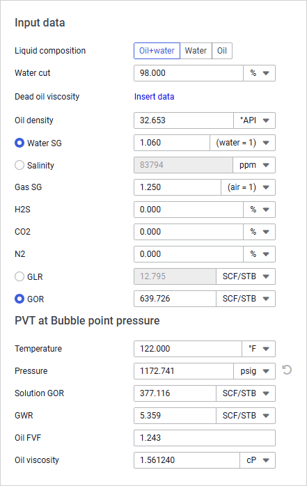
The pane contains PVT property values distributed in two parameter groups:
- Input data: Parameter values at standard conditions.
To configure dead oil viscosity matching, to the right of the parameter name, click Insert data. For details, see Configuring Dead Oil Viscosity Matching. - PVT at bubble point pressure: Parameter values at a specified temperature.
The temperature is specified in the Temperature field.
Visualization of the PVT properties at this temperature is displayed in the left part of the tab (see description below).
Visualization Pane
The pane contains charts that visualize the FVF, Solution GOR, and Viscosity values of oil, water, and gas at the temperature specified in the Temperature field in the configuration pane (see description above).
The pane consists of three tabs with charts of the corresponding fluid components:
- Oil properties at X °C
- Water properties at X °C
- Gas properties at X °C
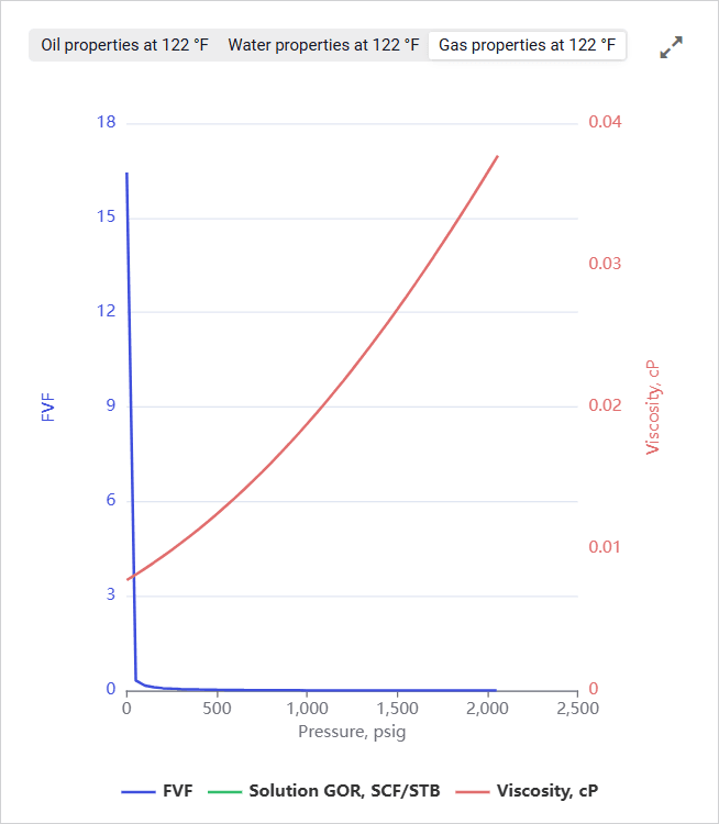
To show or hide a parameter on the chart, click the parameter name under it.
You can also expand the pane to full screen or collapse it back to the original size using the Expand ( ) / Collapse ( ) buttons located in the upper-right corner of the pane.
Configuring Fluid PVT Properties
To configure dead oil viscosity matching, perform the following actions:
- Open the nv.design module.
For details on navigation in the system, see System Interface. - In the left part of the working area, in the list of the module sections, click Fluid.
To the right of the list, the Fluid tab opens.
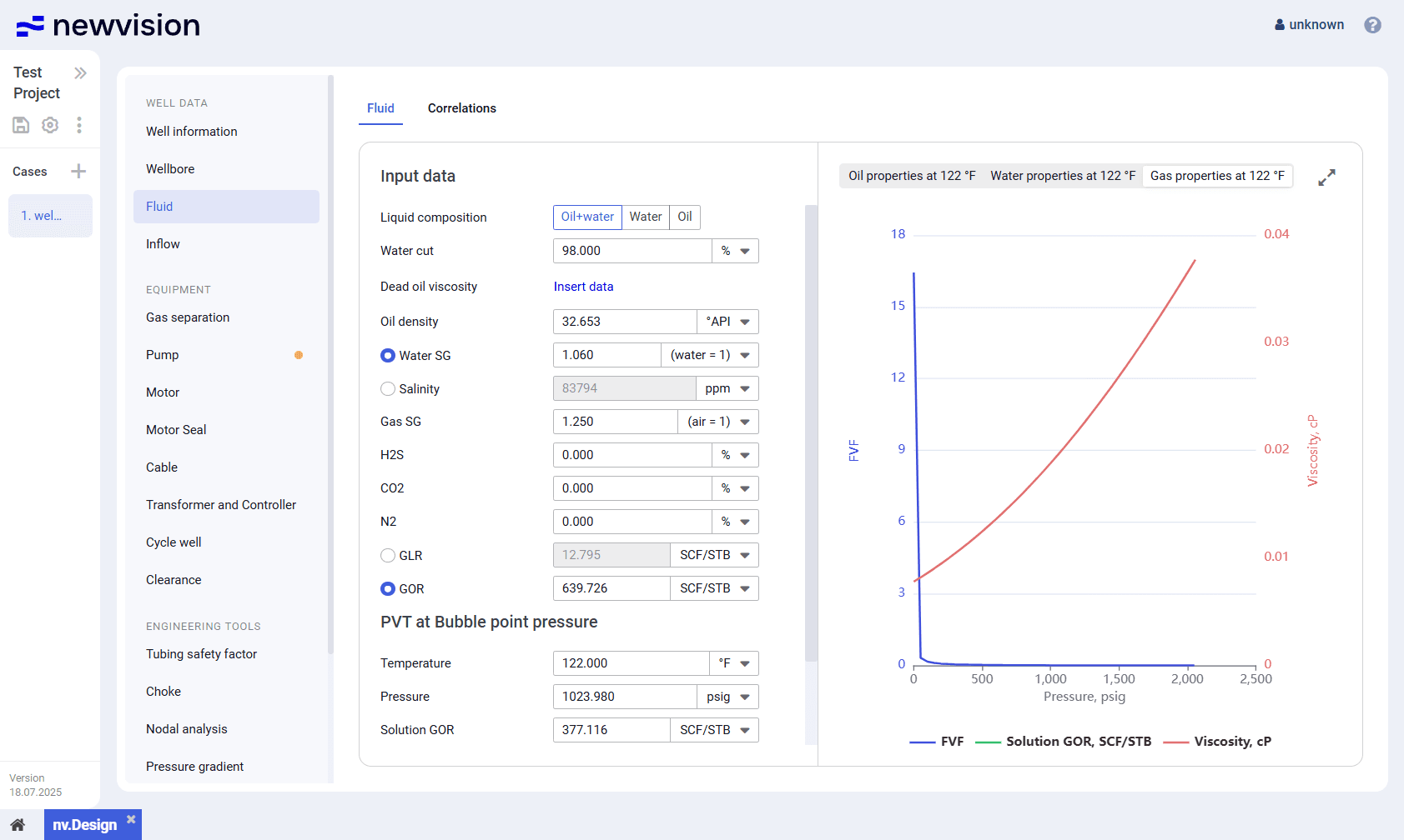
- In the left part of the tab, in the Input data parameter group, perform the following actions:
- To the right of the Liquid composition parameter name, select the well fluid composition option: Oil+water, Water, or Oil.
In the list of available parameters below, only the parameters relevant to the selected composition remain. - In the Water cut field, enter the desired value.
- (Optional) If the fluid composition includes high-viscosity oil, click Insert data and configure matching parameters so that available correlations could be applied. For details, see Dead Oil Viscosity Matching.
| Note |
- In the Input data parameter group, fill in the rest of the PVT properties under surface conditions.
Go to the Correlations tab and select the correlations that are most suitable for the input parameters. For details, see Appendix A: PVT Correlations. - Parameter values in the PVT at Bubble point pressure group are calculated automatically based on the selected correlations.
- (Optional) Edit values in the PVT at Bubble point pressure group.
| Note  |
- In the right part of the tab, view charts that visualize the FVF, Solution GOR, and Viscosity values of gas, water, and/or oil at the temperature specified in the Temperature field.
To save changes, in the left part of the module, click Save ( ) under the name of the current project.
Dead Oil Viscosity Matching
To configure dead oil viscosity matching, perform the following actions:
- Open the nv.design module.
For details on navigation in the system, see System Interface. - In the left part of the working area, in the list of the module sections, click Fluid.
To the right of the list, the Fluid tab opens.
- In the left part of the tab, under the Input data heading, click Insert data.
| Note |
- The Dead oil viscosity window opens in the right part of the tab.
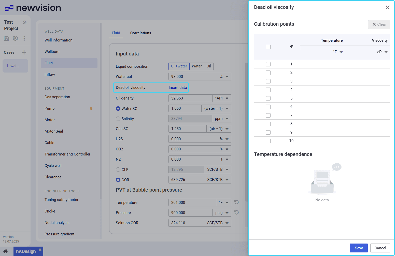
- In the window, add matching data to the Calibration points table. You can do it in the following ways:
- To add data manually, double-click cells in the Temperature and Viscosity columns and enter the desired values.
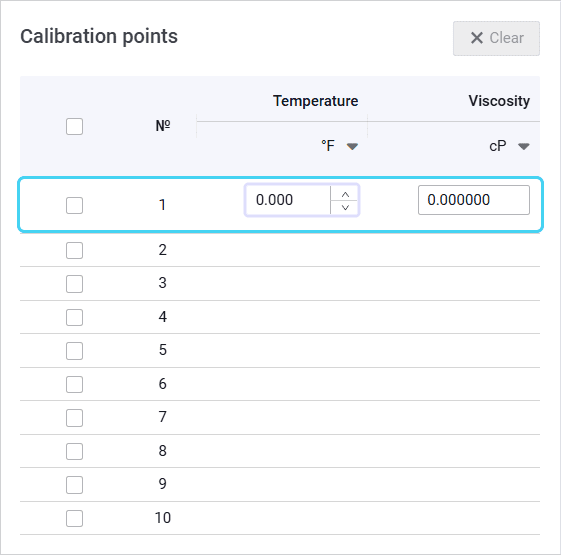
- To paste data from another table, copy it to the clipboard, and then press Ctrl+V.
The copied entries appear in the table. The more data you add, the more accurate results the matching provides.
| Note |
- (Optional)
- To edit values in the table, double-click the desired value and make necessary changes.
To clear data from a row, select its check box in the leftmost column, and then, above the table, click Clear ( ).

- After the configuration is completed, at the bottom of the window, click Save.
Below the Calibration points table, the Temperature dependence chart appears. Under the PVT at Bubble point pressure heading in the left part of the tab, the Oil viscosity value is matched to the actual data.
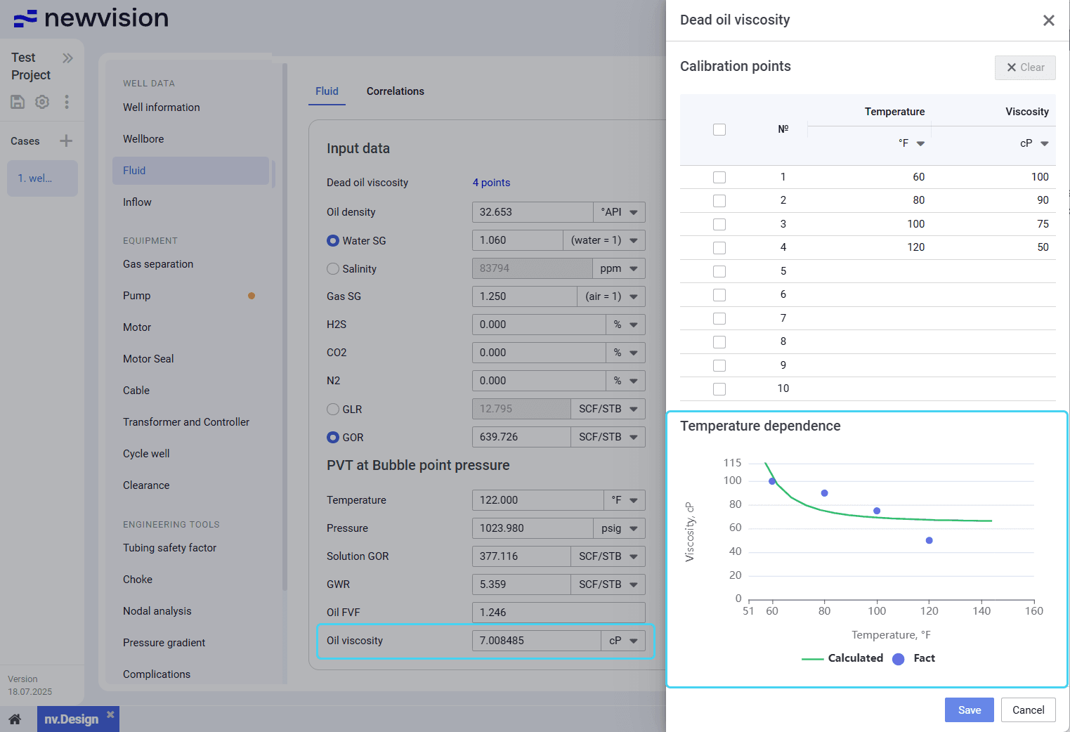
Close the window by clicking the cross icon ( ) in its upper-right corner.
To save changes, in the left part of the module, click Save ( ) under the name of the current project.
Correlations
On the Correlations tab, you can select correlations that are used for the PVT property calculations.
The tab consists of two panes:
- Correlations pane in the left part of the tab.
- Visualization pane in the right part of the tab.
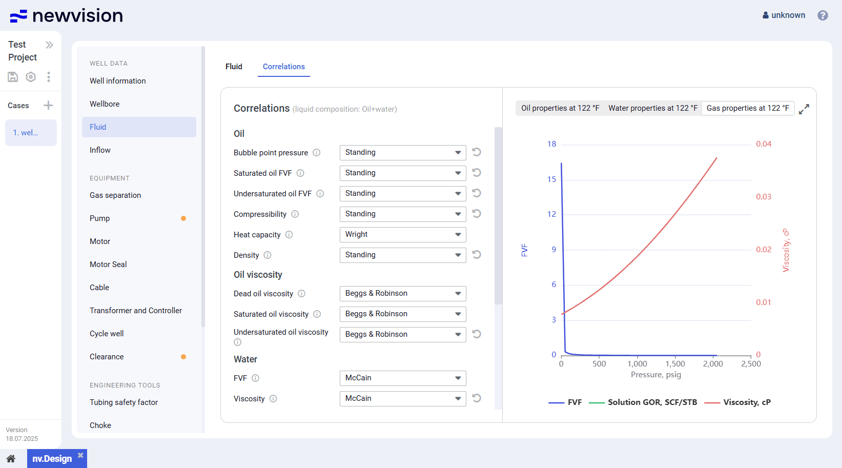
In addition to the basic physical properties of oil, gas, and water, you can configure the interfacial tension between gas and water, as well as between gas and oil. Interfacial tension affects the flow regime, phase slip, and emulsion formation in multi-phase flow, which in turn impacts pressure and velocity calculations.
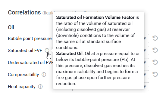
Next to the names of available parameters, the information icon ( ) is displayed. On hovering over it, a hint with a brief description of the corresponding parameter appears.

| Note |
In the right part of the tab, the same visualization pane is displayed. For details, see Fluid.
A detailed description of the correlations and the criteria for their selection are provided in Appendix A: PVT Correlations.
Inflow
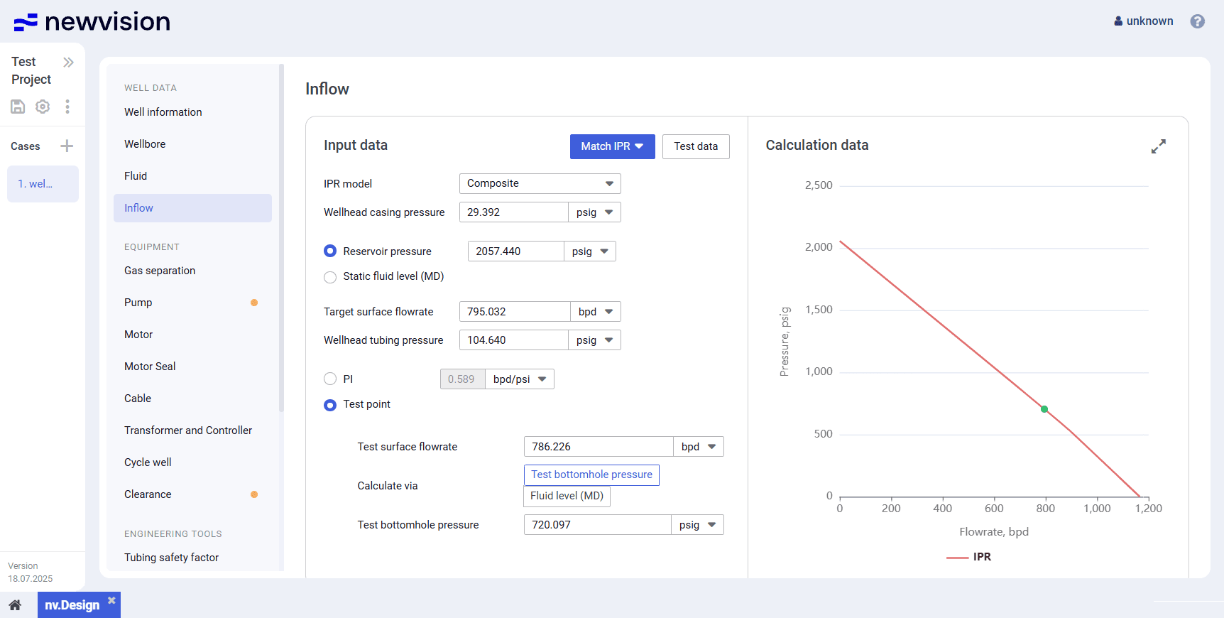
The section provides information about the well inflow parameters that are used for building the IPR (Inflow Performance Relationship) curve.
The section consists of two panes:
- Input data
- Calculation data
Input Data
The pane contains the well parameters used for the IPR construction.
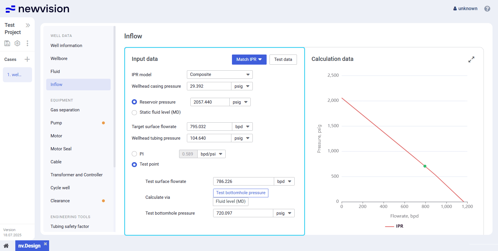
The IPR configuration depends on the model that is used for calculation. The choice of the model should be determined by the reservoir type, well operating conditions, analysis goals, and available data.
For details on the IPR configuration, see Calculating IPR.
You can select one of the following models from the IPR model list:
Composite
This model combines several inflow models and is applied under complex operating conditions: high water cut (above 40–50%), multiphase flow (oil, water, gas), varying inflow regimes, and reservoir heterogeneity.
This approach requires a more comprehensive dataset but provides a more realistic estimate of well performance, especially when bottomhole pressure significantly deviates from bubble point pressure and phase transitions or inflows from different reservoir zones occur.
Vogel Model
This model assumes homogeneous flow (typically oil) and is most effective when bottomhole pressure is below bubble point pressure with minimal water production. It accounts for gas liberation due to pressure drop and provides reliable inflow prediction for undersaturated reservoirs.
However, the model’s accuracy decreases with high water cut. In this case, the composite model is preferred. The PI model is not suitable under these conditions, as it fails to account for multiphase effects.
PI (Productivity Index)
This model is based on a linear relationship between flow rate and pressure drawdown and is applicable only when bottomhole pressure is above bubble point pressure and water cut is low.
In the presence of gas release or increasing water production, the model becomes unreliable because it does not reflect phase changes or increased flow resistance under multiphase flow conditions.
The calculation can be based either on the reservoir pressure value or, if it is unavailable, on the static fluid level. You can also select between calculation based on the productivity index (PI) and a set of custom parameters (Test point). For details, see Calculating IPR.
Calculation Data
The pane contains the IPR curve constructed based on the parameter values entered in the Input data pane.
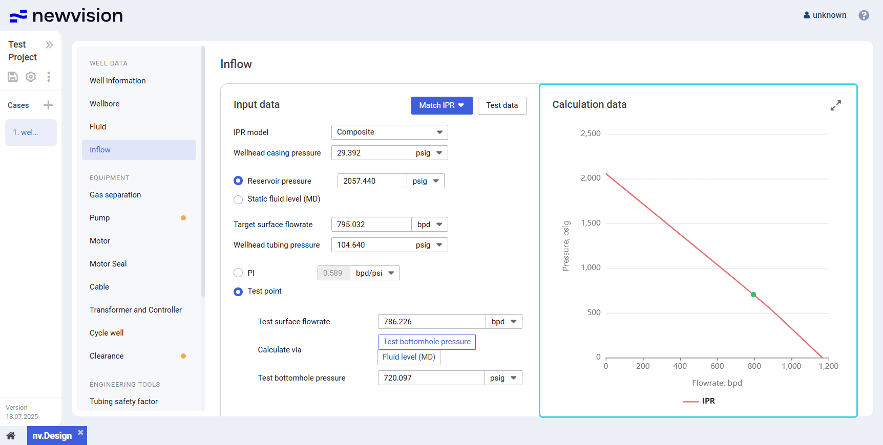
You can expand the pane to full screen or collapse it back to the original size using the Expand ( ) / Collapse ( ) buttons located in the upper-right corner of the pane.
Calculating IPR
To configure deviation survey parameters and run a calculation, perform the following actions:
- Open the nv.design module.
For details on navigation in the system, see System Interface. - In the left part of the working area, in the list of the module sections, click Inflow.
To the right of the list, the Inflow section opens.
- In the upper-right corner of the Input data pane, click Test data.
The Test data window opens.
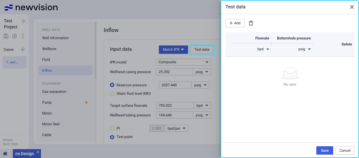
- In the window, enter actual values of the flow rate and corresponding bottom hole pressures obtained during well tests:
Above the table, click Add ( ).
A new row appears in the table.- In the new row, double-click values in the Flowrate and Bottomhole pressure columns and enter the desired values.
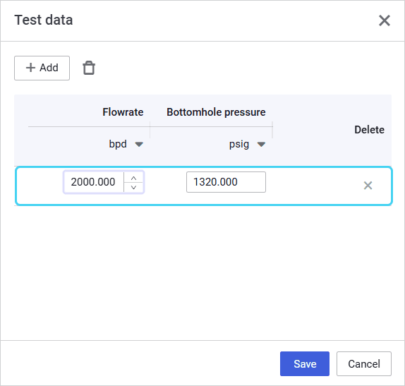
- Repeat Steps 1–2 for all available measurements.
| Note |
- (Optional)
- To edit an entry, double-click the desired value and make necessary changes.
To delete an entry, select it in the table, and then, above the table, click Delete ( ), or click the cross icon ( ) in the Delete column.

- At the bottom of the window, click Save.
- At the top of the Input data pane, from the IPR model list, select the appropriate model: Composite, Vogel, or PI. For description of these models, see .
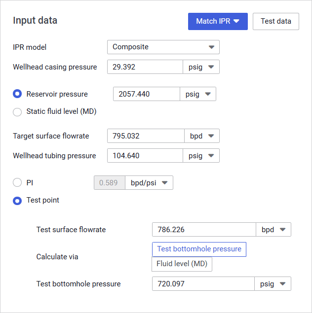
- In the Wellhead casing pressure field, enter the desired value.
- Select the parameter that will be used for the calculation: Reservoir pressure or, if it is unavailable, Static fluid level (MD).
- (Optional) If the Static fluid level (MD) option is selected, fill in the Wellhead casing pressure and Static fluid level (MD) fields.
- In the Target surface flowrate and Wellhead tubing pressure fields, enter the desired target values.
- Select one more parameter based on which the calculation will be performed: productivity index (PI) or a set of custom parameters (Test point).
- Depending on the option selected at the previous step, perform one of the following actions:
- (For PI) In the PI field, enter the productivity index value.
- (For Test point) Fill in the Test surface flowrate field, select the desired Calculate via option, and fill in the rest of the fields.
- In the upper-right corner of the Input data pane, click Match IPR and select PI from the drop-down menu.
In the Calculation data pane, the IPR curve is matched to the actual data and configured calculation parameters. To save changes, in the left part of the module, click Save ( ) under the name of the current project.